Introduction of Optimization#
The optimization serves as an important tool for decision making, resource allocation, and many other applications. Optimization algorithms are widely used in machine learning, statistics, and other fields.
Formulation of Optimization Problems#
An optimization problem can be formulated as follows:
an objective function: \(f(x)\), which is meant to be maximized or minimized
decision variables: \(x \in \mathbb{R}^n\)
constraints: \(g_i(x) \le 0\), \(h_j(x) = 0\)
The standard form of an optimization problem is
The objective is to find the optimal decision variable \(x^*\) that minimizes the objective function \(f(x)\) while satisfying all the constraints.
Definition 1
A feasible solution is a solution that satisfies all the constraints, otherwise, the solution is called infeasible.
The feasible region of an optimization problem is the set of all feasible solutions. The feasible region is also called the feasible set.
In the following, we provide an example to illustrate the concept of the feasible region.
Example 1
We can reformulate the optimization problem with the standard form:
the objective function: \(f(x) = (x_1-2)^2 + (x_2-1)^2\)
decision variables: \(x = (x_1, x_2)\)
constraints: \(g_1(x) = x_1^2 - x_2 \le 0\), \(g_2(x) = x_1 + x_2 \le 2\)
The following code snippet shows the feasible region of the optimization problem.
import matplotlib.pyplot as plt
import numpy as np

%matplotlib inline

# Construct the feasible region
x = np.linspace(-3, 3, 2000)

y1 = x**2
y2 = 2 - x

plt.plot(x, y1, label=r'$x_2 - x_1^2\geq 0$')
plt.plot(x, y2, label=r'$2 - x_1 -x_2\geq 0$')
plt.xlim((-3, 3))
plt.ylim((0, 6))
plt.xlabel(r'$x_1$')
plt.ylabel(r'$x_2$')
plt.fill_between(x, y2, y1, where=y2>y1, color='grey', alpha=0.5)
plt.legend(bbox_to_anchor=(1.05, 1), loc=2, borderaxespad=0.)
<matplotlib.legend.Legend at 0x7fd919a819a0>

Continuous vs. Discrete Optimization#
Some optimization problems have special requirements on the decision variables. For example, the decision variables are required to be integers or discrete values, then the optimization problem is called discrete optimization. Otherwise, the optimization problem is called continuous optimization.
The discrete optimization problems are usually more difficult to solve than continuous optimization problems. The discrete optimization problems are widely used in combinatorial optimization, such as the traveling salesman problem, the knapsack problem, and the assignment problem.
Unconstrained vs. Constrained Optimization#
Optimization problems can be classified into two categories: unconstrained optimization and constrained optimization.
Unconstrained optimization: the optimization problem does not have any constraints or it is safe to ignore the constraints. Sometimes constrained optimization problems can be converted into unconstrained optimization problems by using the Lagrange multiplier method.
Constrained optimization: the optimization problem has constraints, for instance, \(g_i(x) \le 0\), \(h_j(x) = 0\). The constraints can be linear or nonlinear, equality or inequality.
Global vs. Local Optimization#
Most fast optimization algorithms can only find a local minimum, which is not necessarily the global minimum. The global optimization problem is usually more difficult to solve than the local optimization problem. The global optimization problem is also called the global optimization.
One special case of the global optimization problem is the convex optimization problem, whose local minimums are also global minimums. The convex optimization problem is usually easier to solve than the general optimization problem.
Optimization Algorithms#
Most optimization algorithms are iterative algorithms, which means they start from an initial point \(x_0\in\mathbb{R}^n\) and then generate a sequence of points \(x_k\), \(k=1,2,\cdots\) that converge to the optimal solution. The sequence of points is called the iterative sequence.
Ideally, a perfect algorithm should have the following properties:
Robustness: the algorithm should be able to handle different types of optimization problems, such as convex, non-convex, smooth, non-smooth, etc.
Efficiency: the algorithm should be able to find the optimal solution within a reasonable amount of time.
Accuracy: the algorithm should be able to find the optimal solution with high precision.
These properties are usually conflicting with each other. For example, a rapidly convergent algorithm for nonlinear programming may require too much computation resources on large problems. On the other hand, a robust algorithm may also be the slowest one. The trade-off between these properties is a key issue in the design of optimization algorithms.
Convexity#
The convexity plays an important role in optimization. Usually it implies some benign properties of the optimization problem. The convexity applies to both sets and functions.
For sets, a set \(C\subseteq\mathbb{R}^n\) is called convex if the line segment between any two points in \(C\) is also in \(C\). Mathematically, it means
\[\lambda x + (1-\lambda)y\in C, \quad \forall x, y\in C,\quad \lambda\in[0,1].\]For functions, a function \(f(x)\) is called convex if its domain is a convex set and the following inequality holds
\[f(\lambda x + (1-\lambda)y) \le \lambda f(x) + (1-\lambda)f(y), \quad \forall x, y\in\text{dom}f,\quad \lambda\in[0,1].\]
A function \(f\) is called concave if \(-f\) is convex. A function \(f\) is called strictly convex if the inequality is strict.
Convex programming is a special case of mathematical optimization in which
the objective function is convex.
the equality constraints are affine.
the inequality constraints are convex.
Fundamentals of unconstrained optimization#
In unconstrained optimization, we minimize a function \(f(x)\) without any constraints. An typical optimization problem can be formulated as
where \(x\in\mathbb{R}^n\) is the decision variable with \(n\ge 1\) and \(f:\mathbb{R}^n\to \mathbb{R}\) is a smooth objective function.
The following linear regression example illustrates an unconstrained optimization problem.
import numpy as np
import matplotlib.pyplot as plt
import timeit

%matplotlib inline

np.random.seed(0)
N = 100
x = np.random.rand(N)
y = x + 0.5 * (2 * np.random.rand(N) - 1)
plt.scatter(x, y, c='red', marker='^')
<matplotlib.collections.PathCollection at 0x7fd9185b7a90>
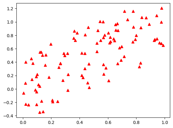
The objective is to find the best linear fit of the data points. The linear regression problem can be formulated as a least square problem, which is an unconstrained optimization problem. The objective function is
from scipy.optimize import leastsq

def residual(p):
    global x, y
    return p[0] * x + p[1] - y

p0 = [5, 5]
z_opt = leastsq(residual, p0, xtol=1e-8, ftol=1e-8)

plt.scatter(x, y, s = 20, c='red', marker='^', label='Data')
plt.scatter(x, z_opt[0][0] * x + z_opt[0][1], s=20, c='b', marker='o', label='Fitted line')
plt.legend(loc='best')
<matplotlib.legend.Legend at 0x7fd90c78fa90>

Global and local minimizer#
The global and local minimizer are important concepts in optimization.
A point \(x^*\) is called a global minimizer of \(f(x)\) if \(f(x^*)\le f(x)\) for all \(x\in\mathbb{R}^n\).
A point \(x^*\) is called a local minimizer of \(f(x)\) if there exists a neighborhood \(N(x^*)\) such that \(f(x^*)\le f(x)\) for all \(x\in N(x^*)\) with \(x\ne x^*\).
A function may have multiple local minimizers. It is usually difficult to locate the global minimizer, it is because the algorithms tend to be attracted to the local minimizers. Sometimes additional assumptions about \(f\) may help to locate the global minimizer.
For twice differentiable functions, a necessary condition for a local minimizer is that the gradient is zero. The second derivative test can be used to determine whether a stationary point is a local minimizer or not.
The sufficient condition for \(x^*\) to be a local minimizer is
\(\nabla f(x^*)=0\), i.e., the first order necessary condition.
\(\nabla^2 f(x^*)\) is positive definite, i.e., the second order sufficient condition.
A strictly local minimizer may fail to satisfy the second order sufficient condition.
Example 2
Consider the function \(f(x) = x^4\). The first derivative is zero at \(x=0\), but the second derivative is zero at \(x=0\). The point \(x=0\) is a local minimizer but not a strict local minimizer.
Two strategies: line search and trust region#
To decide how to move from \(x_k\) to \(x_{k+1}\), the algorithms usually require the information of \(f\) at earlier points. Here we introduce two classical strategies for optimization algorithms: line search and trust region.
Line search: the line search strategy selects a direction \(p_k\) and then searches along this direction from the current point to minimize the objective function. The distance to move is determined by the following one-dimensional optimization problem
\[\min_{\alpha>0} f(x_k + \alpha p_k).\]Here \(\alpha\) is called the step length. The above minimization can be sometimes very expensive to arrive at the exact solution and it is also unnecessary to obtain such an exact solution in practice. The practical line search algorithm will generate a finite number of trial step lengths until it finds a satisfactory one.
The line search strategy is widely used in the optimization algorithms, such as the steepest descent method, the Newton method, the quasi-Newton method, etc.
Trust region: the trust region method does not optimize the objective function directly. Instead, it considers an approximated yet simple model \(m_k\) of the objective function, whose behavior near the current point \(x_k\) is similar to the objective function. Since the model \(m_k\) may not be a good approximation of \(f\) away from \(x_k\), we need to restrict the search for a minimizer of \(m_k\) to a small region around \(x_k\). Mathematically, we are optimizing the following problem
\[\min_{p_k} m_k(x_k + p_k), \quad \text{subject to } \|p_k\|\le \Delta_k,\]where \(\Delta_k\) is called the trust region radius. The trust region method is widely used in the optimization algorithms, such as the trust region Newton method, the trust region conjugate gradient method, etc.